$R2r\pm6p$

R Tour in about 6 pages

Readr, Tidyr, Dplyr

Tidyverse R

                                          
read ->

readr

Tidyverse R

                                          
read -> wrangle

tidyr

Tidyverse R

                                         
read -> wrangle ------> transform

dplyr

Tidyverse R

                                          
read -> wrangle ------> transform ---.
                                     |            
                                     v
                             visualize

ggplot2

Tidyverse R

                                        
read -> wrangle ------> transform ---.
                                     |            
                                     v
                   model <-- visualize

ez
afex
emmeans
effectsize
bayesfactor
rstan

Tidyverse R

                                          
read -> wrangle ---.--> transform ---.
                   ^                 |            
                   |                 v
                   model <-- visualize

xtable
rmarkdown
kableExtra
broom

Tidyverse R

                                          .---> Communicate
read -> wrangle ---.--> transform ---+-- /
                   ^                 |            
                   |                 v
                   model <-- visualize

knitr
rstudio notebook
quarto
bookdown
blogdown
papaja
gtsummary

Sources & Recommended Reading

rstudio-education.github.io/hopr/

r4ds.had.co.nz

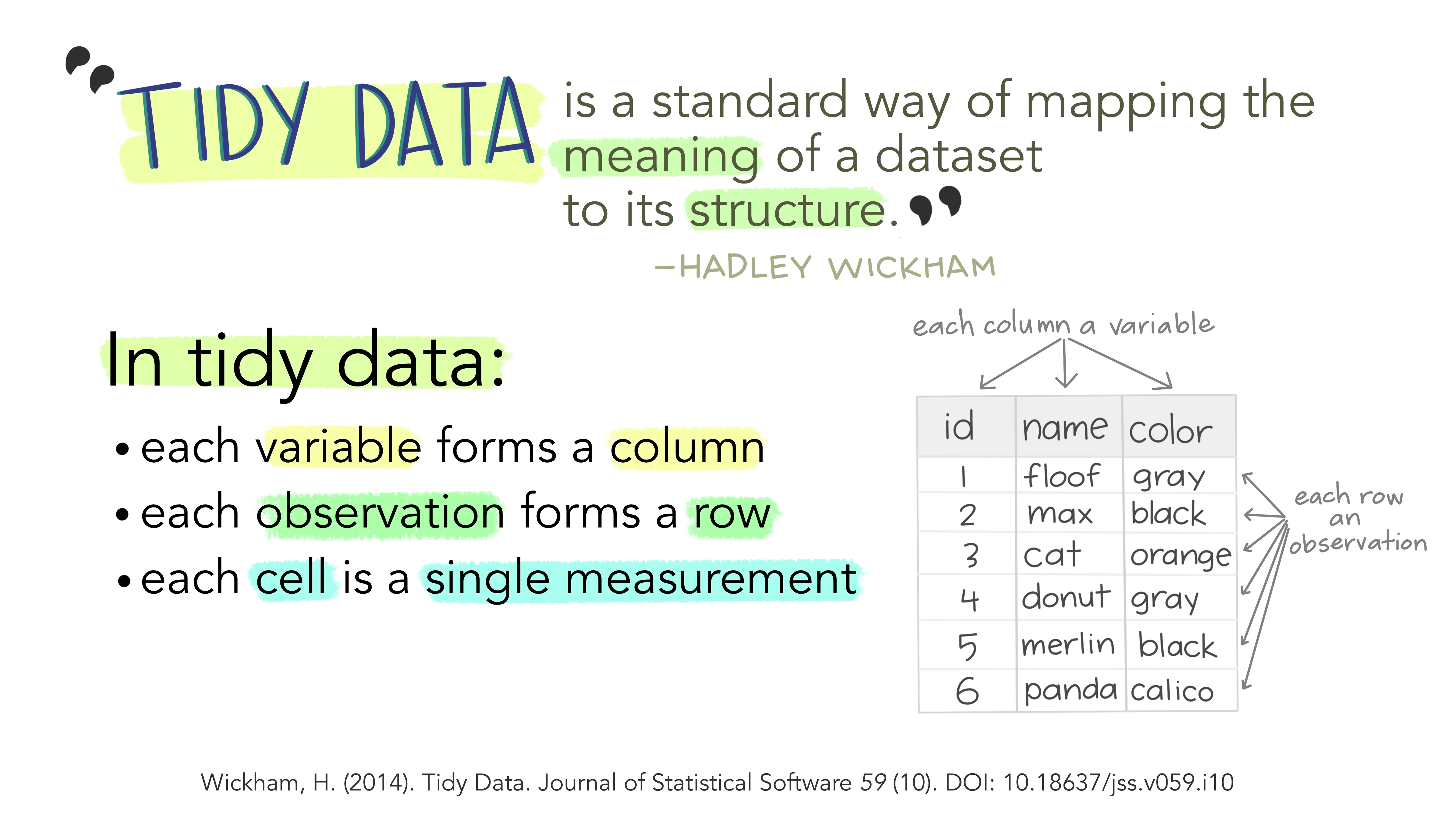
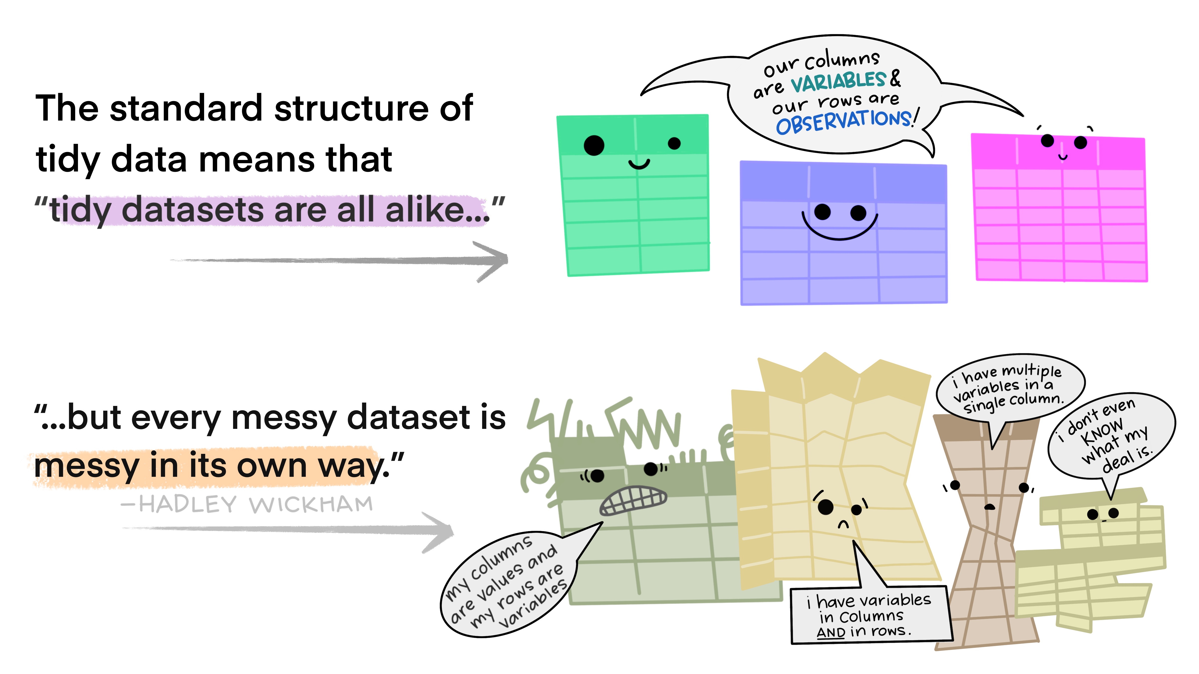
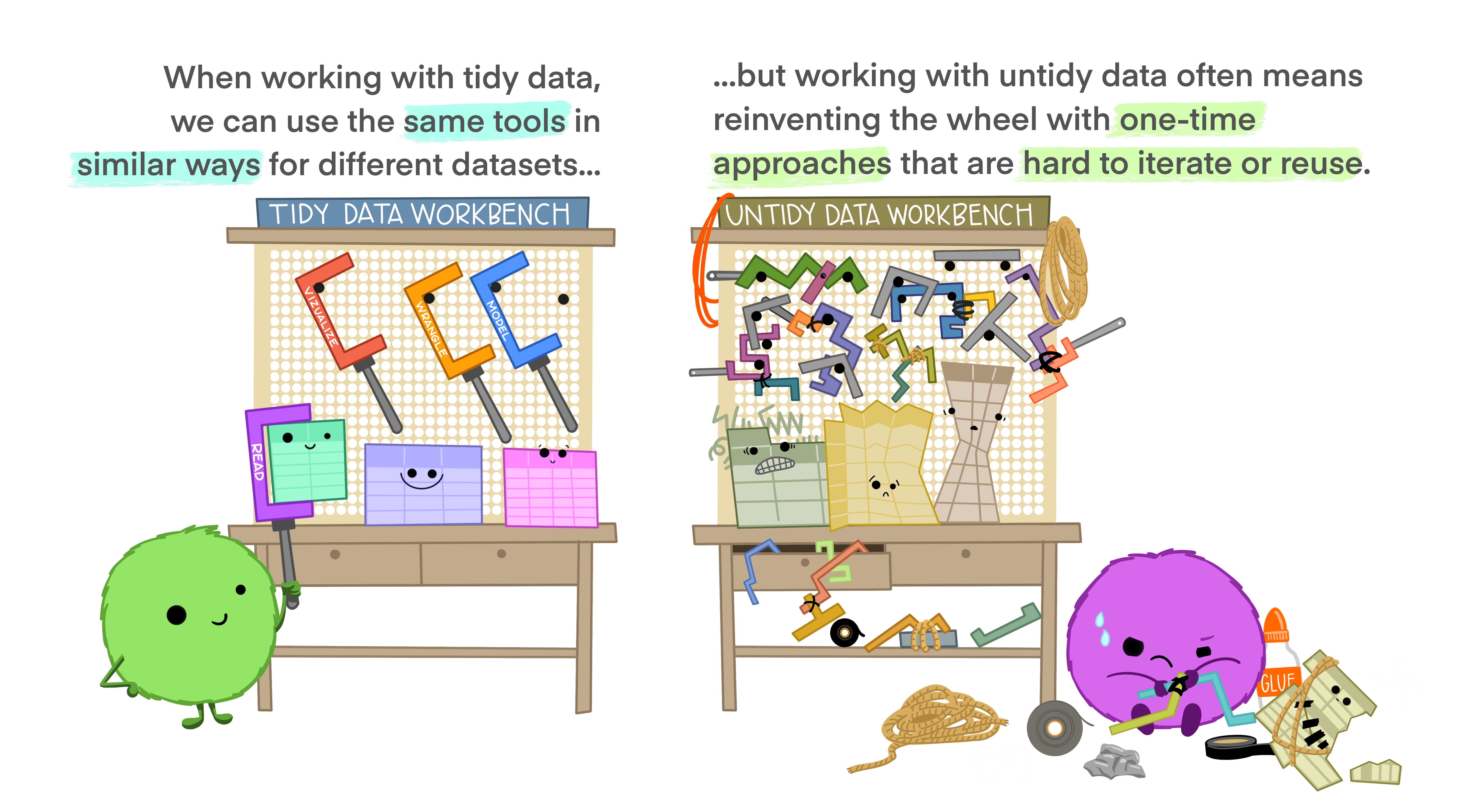
Tidyverse in a Nutshell

  Tidyverse is a set of packages with methods to
      form and to work with rectangular data (variables x cases).
  Data-frames have variables as columns & cases as rows.

Tidyverse Concepts

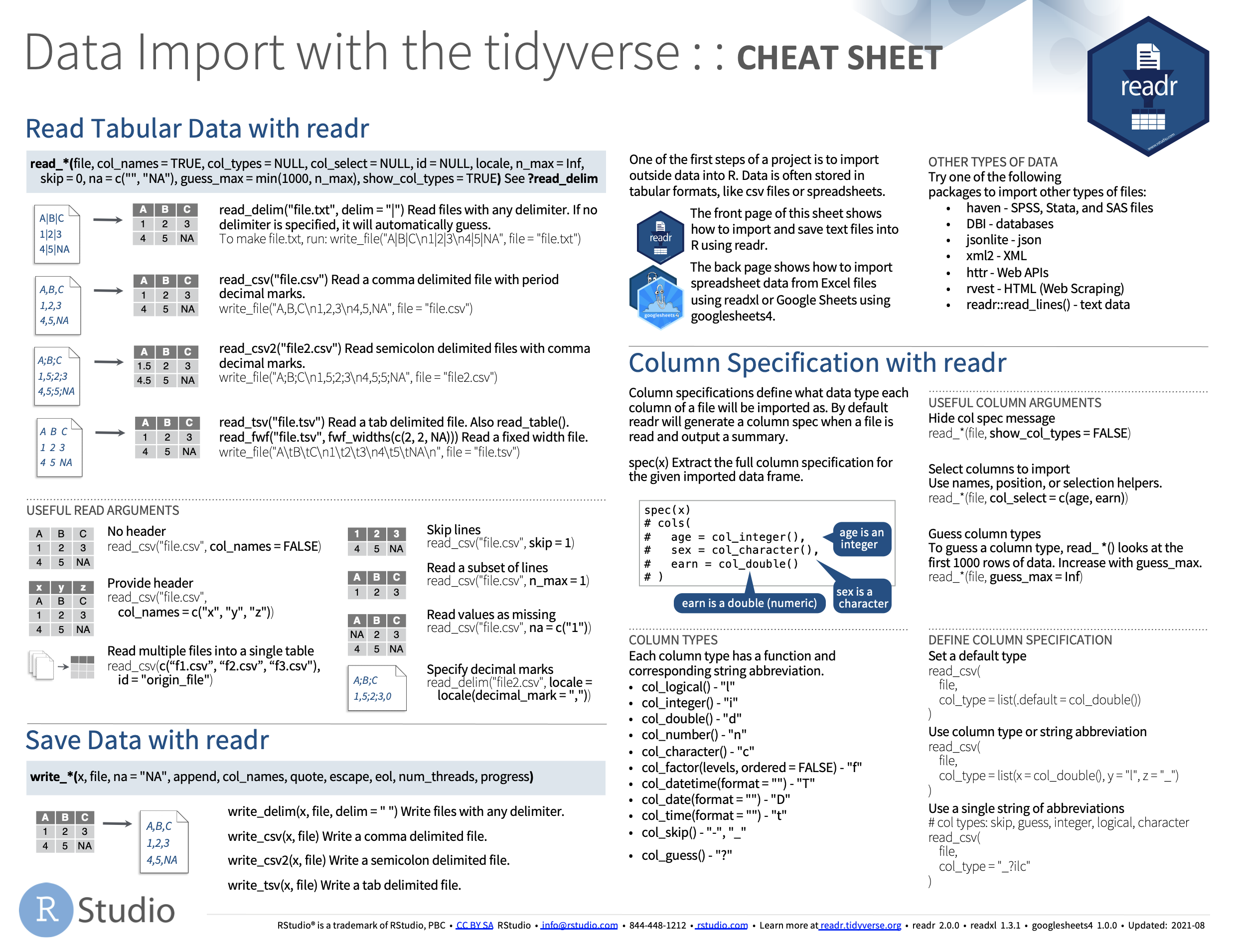
Importing Data with readr

Readr

Tidy Dataframes with tidyr

Tidyr

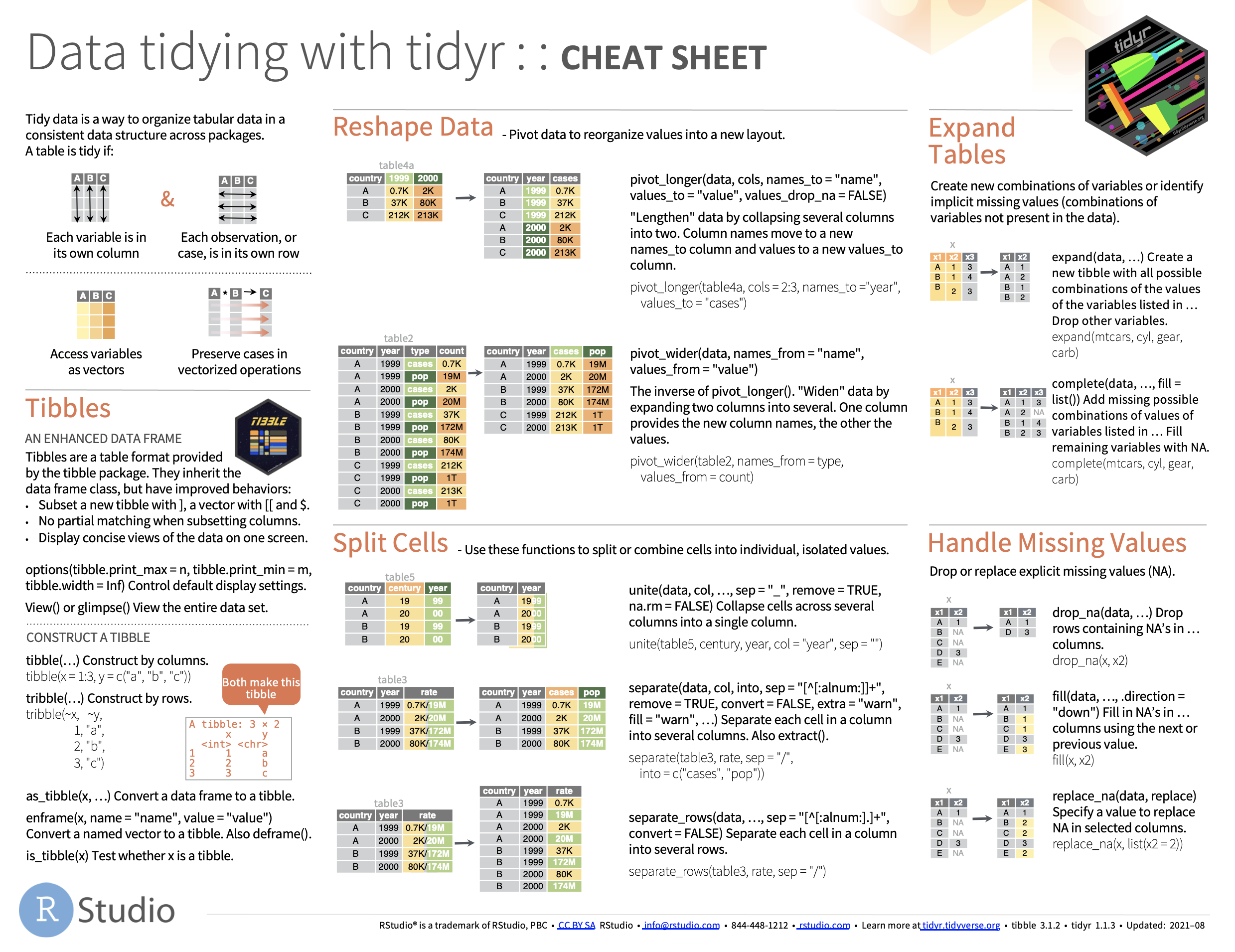
Tibble (an enhanced R dataframe)

Tibbles are a table format provided by the tibble package.
They inherit the data frame class, but have improved behaviors:
- Subset a new tibble with ], a vector with [[ and $.
- No partial matching when subsetting columns.
- Display concise views of the data on one screen.

Tidyr: Reshape data with pivot_longer

pivot longer: Pivot data to reorganize values into a new layout.

“Lengthen” data by collapsing several columns into two.
Column names move to a new
names_to column and values
to a new values_to column.

country	1999	2000
Afghanistan	745	2666
Brazil	37737	80488
China	212258	213766

pivot_longer(table4a, cols = 2:3, 
             names_to ="year", 
             values_to = "cases")

country	year	cases
Afghanistan	1999	745
Afghanistan	2000	2666
Brazil	1999	37737
Brazil	2000	80488
China	1999	212258
China	2000	213766

Tidyr: Reshape data with pivot_wider

pivot_wider: inverse of pivot_longer().

“Widen” data by expanding two columns into several.
One column provides a new column, names, the other, values.

country	year	type	count
Afghanistan	1999	cases	745
Afghanistan	1999	population	19987071
Afghanistan	2000	cases	2666
Afghanistan	2000	population	20595360
Brazil	1999	cases	37737
Brazil	1999	population	172006362
Brazil	2000	cases	80488
Brazil	2000	population	174504898
China	1999	cases	212258
China	1999	population	1272915272
China	2000	cases	213766
China	2000	population	1280428583

pivot_wider(table2, 
            names_from = type,
            values_from = count
            )

country	year	cases	population
Afghanistan	1999	745	19987071
Afghanistan	2000	2666	20595360
Brazil	1999	37737	172006362
Brazil	2000	80488	174504898
China	1999	212258	1272915272
China	2000	213766	1280428583

Tidyr: unite

*unite(data, col, …, sep = “_“, remove = TRUE, na.rm = FALSE)*

Collapse cells across several columns into
a single column.

country	century	year	rate
Afghanistan	19	99	745/19987071
Afghanistan	20	00	2666/20595360
Brazil	19	99	37737/172006362
Brazil	20	00	80488/174504898
China	19	99	212258/1272915272
China	20	00	213766/1280428583

unite(table5, 
      century, year, 
      col = "year", 
      sep = "")

country	year	rate
Afghanistan	1999	745/19987071
Afghanistan	2000	2666/20595360
Brazil	1999	37737/172006362
Brazil	2000	80488/174504898
China	1999	212258/1272915272
China	2000	213766/1280428583

Tidyr: separate

separate(data, col, into, sep = “[^[:alnum:]]+”, remove = TRUE, convert = FALSE, extra = “warn”, fill = “warn”, …)

Separate each cell in a column into
several columns.
Also extract().

country	year	rate
Afghanistan	1999	745/19987071
Afghanistan	2000	2666/20595360
Brazil	1999	37737/172006362
Brazil	2000	80488/174504898
China	1999	212258/1272915272
China	2000	213766/1280428583

separate(table3, 
         rate, 
         sep = "/",
         into = c("cases", "pop")
         )

country	year	cases	pop
Afghanistan	1999	745	19987071
Afghanistan	2000	2666	20595360
Brazil	1999	37737	172006362
Brazil	2000	80488	174504898
China	1999	212258	1272915272
China	2000	213766	1280428583

Tidyr: separate_rows

separate_rows(data, …, sep = “[^[:alnum:].]+”, convert = FALSE)

Separate each cell in a column into several rows.

country	year	rate
Afghanistan	1999	745/19987071
Afghanistan	2000	2666/20595360
Brazil	1999	37737/172006362
Brazil	2000	80488/174504898
China	1999	212258/1272915272
China	2000	213766/1280428583

separate_rows(table3, rate, sep = "/")

country	year	rate
Afghanistan	1999	745
Afghanistan	1999	19987071
Afghanistan	2000	2666
Afghanistan	2000	20595360
Brazil	1999	37737
Brazil	1999	172006362
Brazil	2000	80488
Brazil	2000	174504898
China	1999	212258
China	1999	1272915272
China	2000	213766
China	2000	1280428583

Dataframe transformation with dplyr

Dplyr - p1:

pipe data from functions
manipulate cases (rows)
manipulate variables (columns)

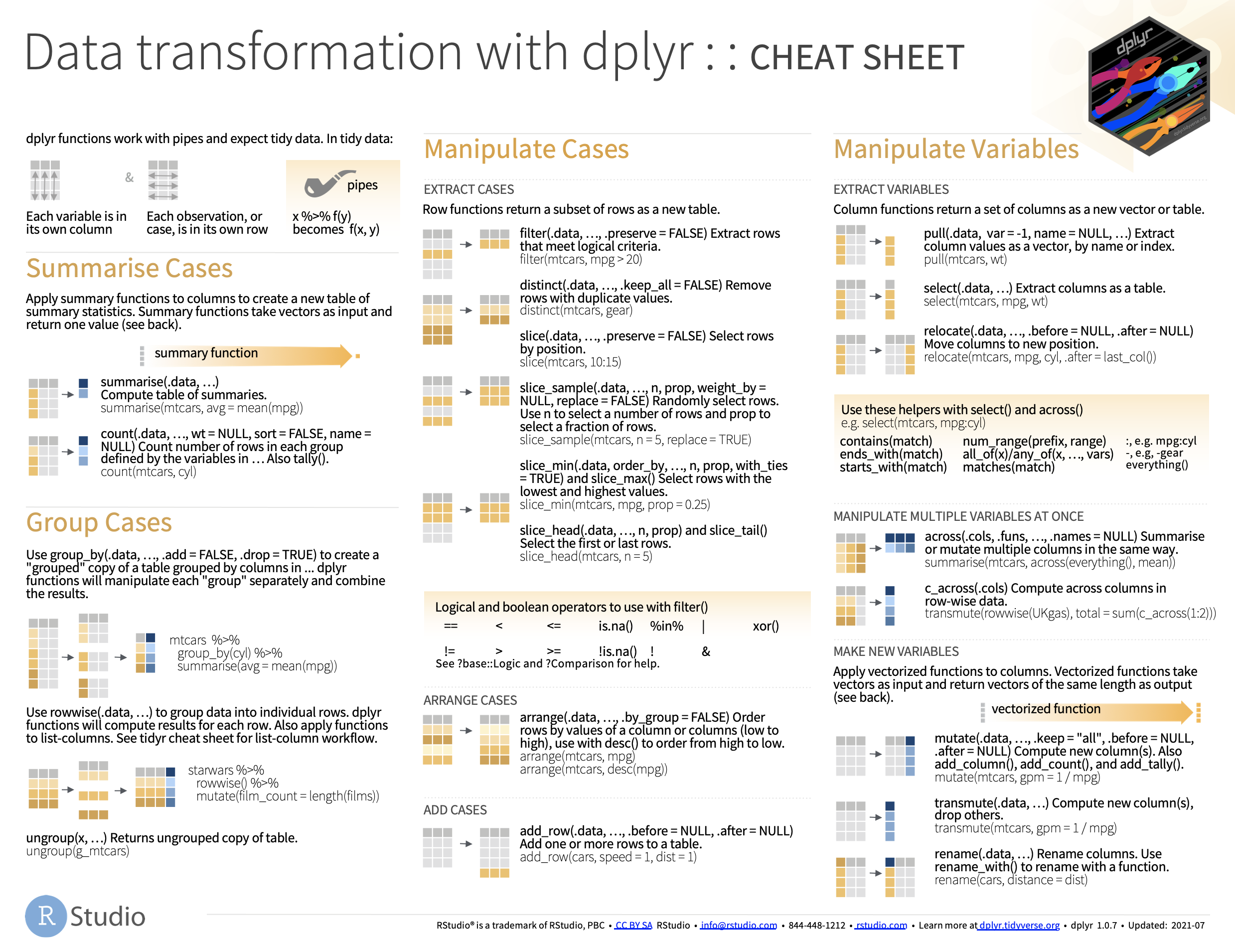
Dplyr: Summarize

summarise(.data, …)

Compute table of summaries.

summarise(mtcars, avg = mean(mpg))

       avg
1 20.09062

count(.data, …, wt = NULL, sort = FALSE, name = NULL)

Count number of rows in each
group defined by the variables in …
Also tally().

starwars %>% 
  count(species,sort = TRUE)

# A tibble: 38 × 2
   species      n
   <chr>    <int>
 1 Human       35
 2 Droid        6
 3 <NA>         4
 4 Gungan       3
 5 Kaminoan     2
 6 Mirialan     2
 7 Twi'lek      2
 8 Wookiee      2
 9 Zabrak       2
10 Aleena       1
# … with 28 more rows

Dplyr: Extract Cases

Row functions return a subset of rows as a new table.

filter(.data, …, .preserve = FALSE)
- Extract rows that meet logical criteria.
- filter(mtcars, mpg > 20)

starwars %>% 
  filter(species == "Droid")

# A tibble: 6 × 14
  name   height  mass hair_color skin_color  eye_color birth_year sex   gender  
  <chr>   <int> <dbl> <chr>      <chr>       <chr>          <dbl> <chr> <chr>   
1 C-3PO     167    75 <NA>       gold        yellow           112 none  masculi…
2 R2-D2      96    32 <NA>       white, blue red               33 none  masculi…
3 R5-D4      97    32 <NA>       white, red  red               NA none  masculi…
4 IG-88     200   140 none       metal       red               15 none  masculi…
5 R4-P17     96    NA none       silver, red red, blue         NA none  feminine
6 BB8        NA    NA none       none        black             NA none  masculi…
# … with 5 more variables: homeworld <chr>, species <chr>, films <list>,
#   vehicles <list>, starships <list>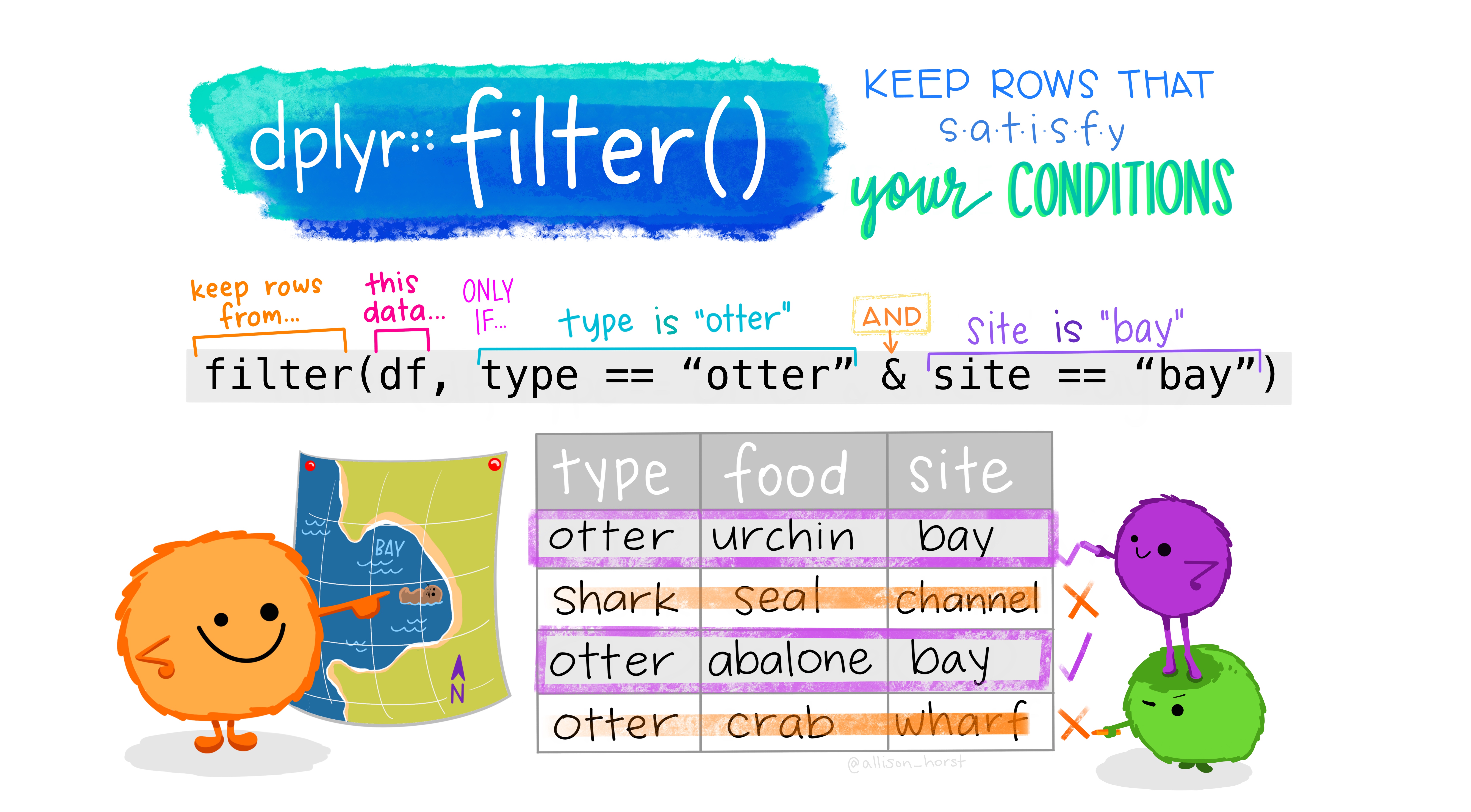

distinct(.data, …, .keep_all = FALSE)
- Remove rows with duplicate values. distinct(mtcars, gear)

starwars %>% 
  distinct(homeworld)

# A tibble: 49 × 1
   homeworld 
   <chr>     
 1 Tatooine  
 2 Naboo     
 3 Alderaan  
 4 Stewjon   
 5 Eriadu    
 6 Kashyyyk  
 7 Corellia  
 8 Rodia     
 9 Nal Hutta 
10 Bestine IV
# … with 39 more rows

Dplyr: Arrange Cases

arrange(.data, …, .by_group = FALSE)
- Order rows by values of a column or columns (low to high), use with desc() to order from high to low.
arrange(mtcars, mpg)
arrange(mtcars, desc(mpg))

starwars %>% 
  mutate(name, bmi = mass / ((height / 100)  ^ 2)) %>%
  select(name:mass, bmi) %>% 
  arrange(desc(bmi))

# A tibble: 87 × 4
   name                  height  mass   bmi
   <chr>                  <int> <dbl> <dbl>
 1 Jabba Desilijic Tiure    175  1358 443. 
 2 Dud Bolt                  94    45  50.9
 3 Yoda                      66    17  39.0
 4 Owen Lars                178   120  37.9
 5 IG-88                    200   140  35  
 6 R2-D2                     96    32  34.7
 7 Grievous                 216   159  34.1
 8 R5-D4                     97    32  34.0
 9 Jek Tono Porkins         180   110  34.0
10 Darth Vader              202   136  33.3
# … with 77 more rows

Dplyr: Manipulate Variables

Extract Variables

Column functions return a set of columns as a new vector or table.

pull(.data, var = -1, name = NULL, …)
- Extract column values as a vector, by name or index.
- pull(mtcars, wt)
select(.data, …)
- Extract columns as a table.
- select(mtcars, mpg, wt)

starwars %>% 
  select(name, ends_with("color"))

# A tibble: 87 × 4
   name               hair_color    skin_color  eye_color
   <chr>              <chr>         <chr>       <chr>    
 1 Luke Skywalker     blond         fair        blue     
 2 C-3PO              <NA>          gold        yellow   
 3 R2-D2              <NA>          white, blue red      
 4 Darth Vader        none          white       yellow   
 5 Leia Organa        brown         light       brown    
 6 Owen Lars          brown, grey   light       blue     
 7 Beru Whitesun lars brown         light       blue     
 8 R5-D4              <NA>          white, red  red      
 9 Biggs Darklighter  black         light       brown    
10 Obi-Wan Kenobi     auburn, white fair        blue-gray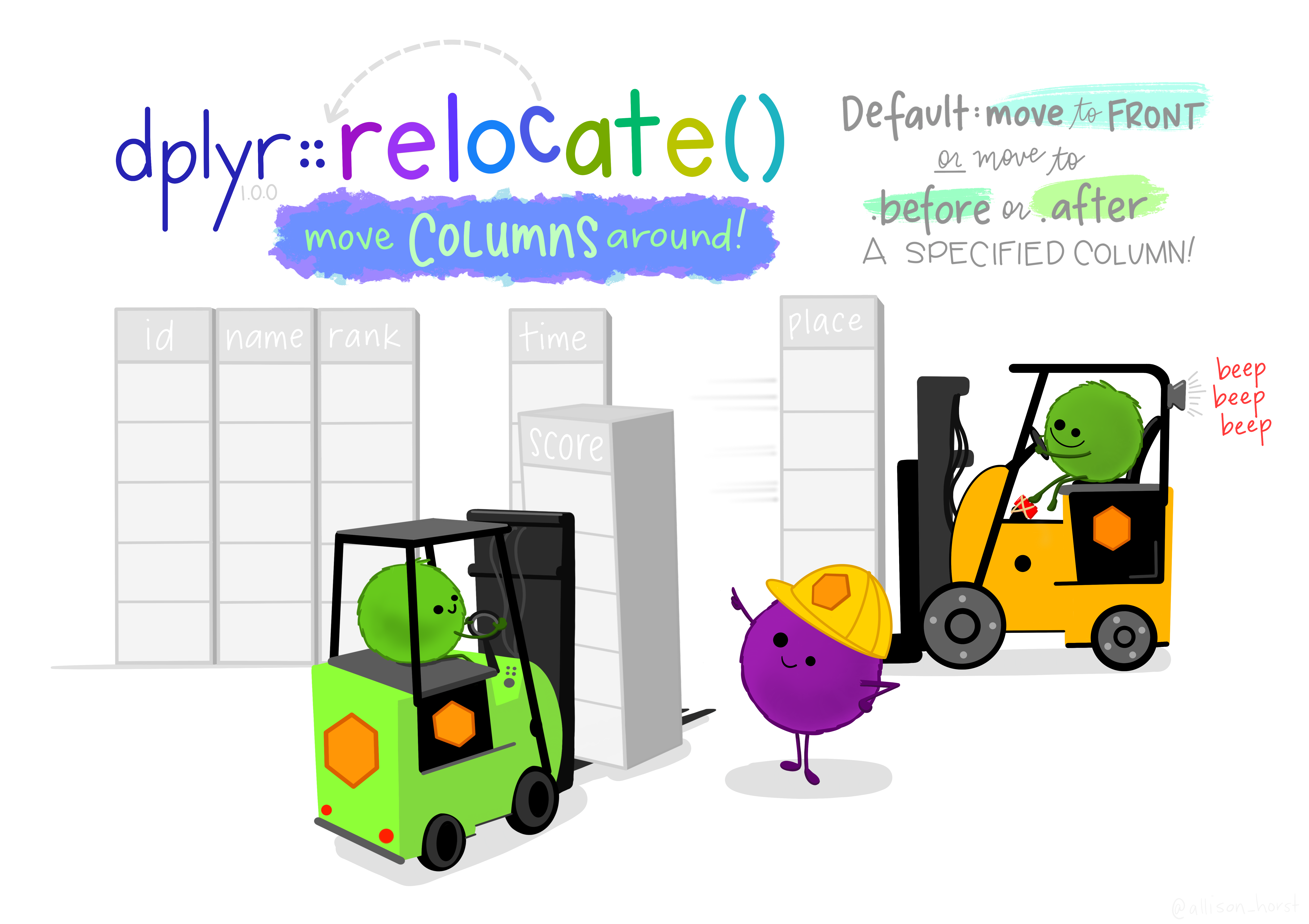
# … with 77 more rows

relocate(.data, …, .before = NULL, .after = NULL)
- Move columns to new position.
- relocate(mtcars, mpg, cyl, .after = last_col())

Dplyr: Manipulate Variables

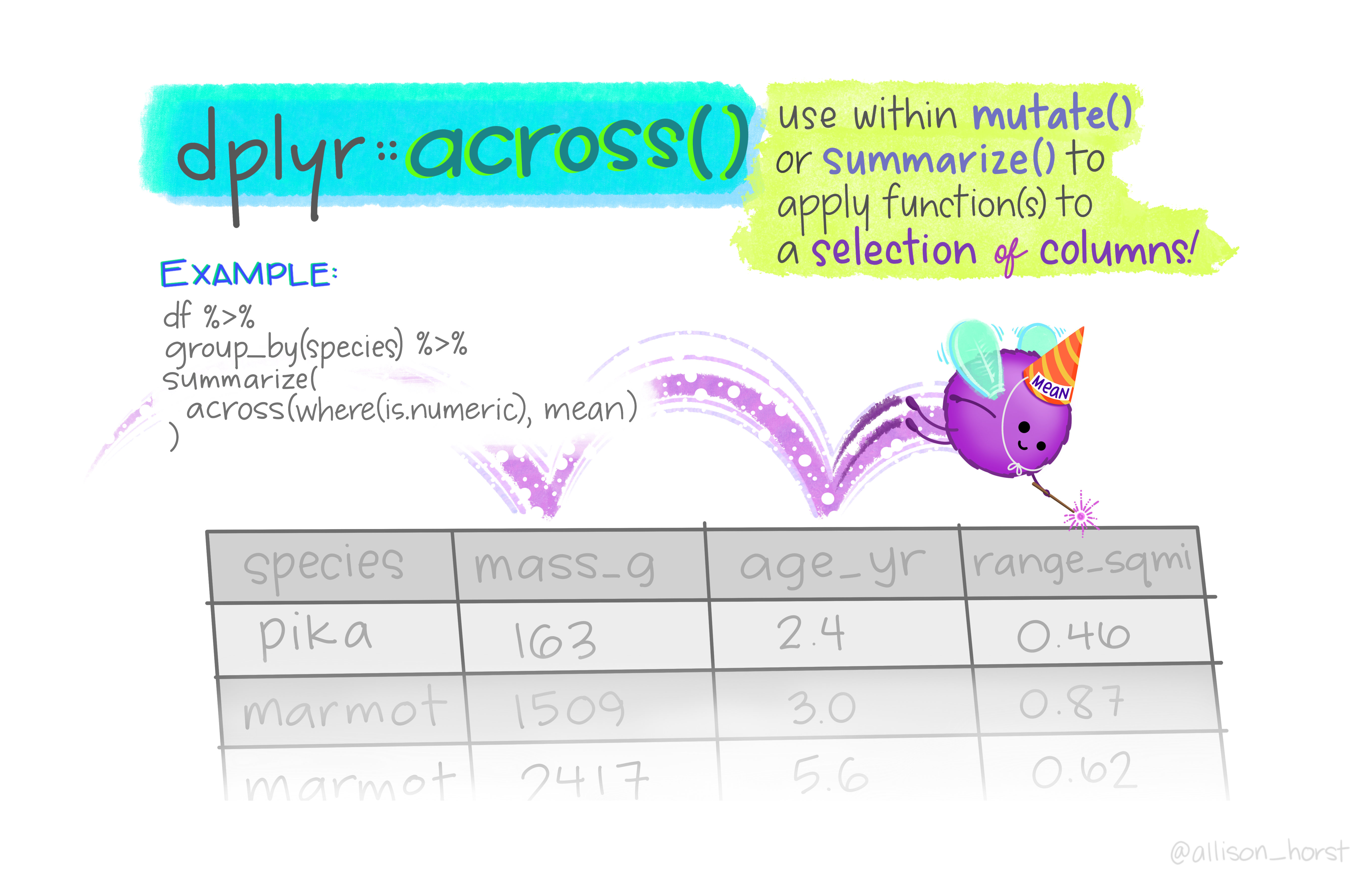
Manipulate multiple variables at once

Use these helpers with select() and across() e.g. select(mtcars, mpg:cyl)

contains(match)
ends_with(match)
starts_with(match)
num_range(prefix, range)
all_of(x)/any_of(x, …, vars)
matches(match)
everything()

Dplyr: Make New Variables

Apply vectorized functions to columns. Vectorized functions take vectors as input and return vectors of the same length as output.

mutate(.data, …, .keep = “all”, .before = NULL, .after = NULL)

Compute new column(s).
add_column(), add_count(), add_tally()
mutate(mtcars, gpm = 1 / mpg)

transmute(.data, …)

Compute new column(s), drop others.
transmute(mtcars, gpm = 1 / mpg)

rename(.data, …)

Rename columns.
Use rename_with() to rename with a function.
rename(cars, distance = dist)

starwars %>% 
  mutate(name, bmi = 
           mass/((height/100)^ 2)) %>%
  select(name:mass, bmi) %>% 
  arrange(desc(bmi))

# A tibble: 87 × 4
   name                  height  mass   bmi
   <chr>                  <int> <dbl> <dbl>
 1 Jabba Desilijic Tiure    175  1358 443. 
 2 Dud Bolt                  94    45  50.9
 3 Yoda                      66    17  39.0
 4 Owen Lars                178   120  37.9
 5 IG-88                    200   140  35  
 6 R2-D2                     96    32  34.7
 7 Grievous                 216   159  34.1
 8 R5-D4                     97    32  34.0
 9 Jek Tono Porkins         180   110  34.0
10 Darth Vader              202   136  33.3
# … with 77 more rows

Mutate

Dplyr: Group Cases

Use group_by(.data, …, .add = FALSE, .drop = TRUE)

to create a “grouped” copy of a table grouped by columns in …
dplyr functions will manipulate each “group” separately and combine the results.

Use rowwise(.data, …) to group data into rows.

dplyr functions will compute results for each row.
Also apply functions to list-columns.
See tidyr cheat sheet for list-column workflow.

ungroup(x, …) Returns ungrouped copy of table.

ungroup(g_mtcars)

starwars %>%
  group_by(species) %>%
  summarise(
    n = n(),
    mass = mean(mass, na.rm = TRUE)
  ) %>%
  filter(n > 1)

# A tibble: 9 × 3
  species      n  mass
  <chr>    <int> <dbl>
1 Droid        6  69.8
2 Gungan       3  74  
3 Human       35  82.8
4 Kaminoan     2  88  
5 Mirialan     2  53.1
6 Twi'lek      2  55  
7 Wookiee      2 124  
8 Zabrak       2  80  
9 <NA>         4  48

Dplyr - p2:

vectorized functions map 1 to 1 from input to output so number of cases (rows) in =’s number out
summary functions output less than #of cases in (combined with group_by() from dplyr p.1 determines number of outputs)
this principle is embodied by the “split-apply-combine” approach
relational joins: straight out of linear algebra and - most of the useful tidyverse meta-programming

Dplyr: Vectorized functions:

work on variables (columns)

dplyr::if_else()

element-wise if() + else()

dplyr::na_if()

replace specific values with NA

starwars %>% 
  mutate(
    cent=if_else(birth_year<100,0,1),
    ) %>% 
  filter(cent==1) %>% 
  select(name,cent,birth_year,species)

# A tibble: 5 × 4
  name                   cent birth_year species       
  <chr>                 <dbl>      <dbl> <chr>         
1 C-3PO                     1        112 Droid         
2 Chewbacca                 1        200 Wookiee       
3 Jabba Desilijic Tiure     1        600 Hutt          
4 Yoda                      1        896 Yoda's species
5 Dooku                     1        102 Human

Dplyr: case_when

dplyr::case_when() - multi-case if_else()

starwars %>% 
  mutate(type = case_when(
    height > 200 | mass > 200 ~ "large",
    species == "Droid"~ "robot",
    TRUE  ~ "other"),
    .before=height
    )

# A tibble: 87 × 15
   name      type  height  mass hair_color skin_color eye_color birth_year sex  
   <chr>     <chr>  <int> <dbl> <chr>      <chr>      <chr>          <dbl> <chr>
 1 Luke Sky… other    172    77 blond      fair       blue            19   male 
 2 C-3PO     robot    167    75 <NA>       gold       yellow         112   none 
 3 R2-D2     robot     96    32 <NA>       white, bl… red             33   none 
 4 Darth Va… large    202   136 none       white      yellow          41.9 male 
 5 Leia Org… other    150    49 brown      light      brown           19   fema…
 6 Owen Lars other    178   120 brown, gr… light      blue            52   male 
 7 Beru Whi… other    165    75 brown      light      blue            47   fema…
 8 R5-D4     robot     97    32 <NA>       white, red red             NA   none 
 9 Biggs Da… other    183    84 black      light      brown           24   male 
10 Obi-Wan … other    182    77 auburn, w… fair       blue-gray       57   male 
# … with 77 more rows, and 6 more variables: gender <chr>, homeworld <chr>,
#   species <chr>, films <list>, vehicles <list>, starships <list>

\(R2r\pm6p\)

Tidyverse R

Tidyverse R

Tidyverse R

Tidyverse R

Tidyverse R

Tidyverse R

Tidyverse R

Sources & Recommended Reading

Tidyverse in a Nutshell

Tidyverse Concepts

Tidyverse Concepts

Tidyverse Concepts

Importing Data with readr

Readr

Tidy Dataframes with tidyr

Tidyr

Tibble (an enhanced R dataframe)

Tidyr: Reshape data with pivot_longer

Tidyr: Reshape data with pivot_wider

Tidyr: unite

Tidyr: separate

Tidyr: separate_rows

Dataframe transformation with dplyr

Dplyr - p1:

Dplyr: Summarize

Dplyr: Extract Cases

Row functions return a subset of rows as a new table.

Dplyr: Arrange Cases

Dplyr: Manipulate Variables

Extract Variables

Dplyr: Manipulate Variables

Manipulate multiple variables at once

Dplyr: Make New Variables

Mutate

Dplyr: Group Cases

Dplyr - p2:

Dplyr - p2:

Dplyr: Vectorized functions:

work on variables (columns)

Dplyr: case_when