<Info | 15 non-empty values
bads: 2 items (MEG 2443, EEG 053)
ch_names: MEG 0113, MEG 0112, MEG 0111, MEG 0122, MEG 0123, MEG 0121, MEG ...
chs: 204 Gradiometers, 102 Magnetometers, 9 Stimulus, 60 EEG, 1 EOG
custom_ref_applied: False
dev_head_t: MEG device -> head transform
dig: 146 items (3 Cardinal, 4 HPI, 61 EEG, 78 Extra)
file_id: 4 items (dict)
highpass: 0.1 Hz
hpi_meas: 1 item (list)
hpi_results: 1 item (list)
lowpass: 40.0 Hz
meas_date: 2002-12-03 19:01:10 UTC
meas_id: 4 items (dict)
nchan: 376
projs: PCA-v1: off, PCA-v2: off, PCA-v3: off, Average EEG reference: off
sfreq: 150.2 Hz
>MNE-Python
Overview: Setup and Load Data
import os
import numpy as np
import mne

sample_data_folder = mne.datasets.sample.data_path()
sample_data_raw_file = os.path.join(sample_data_folder, 'MEG', 'sample',
                                   'sample_audvis_filt-0-40_raw.fif')
raw = mne.io.read_raw_fif(sample_data_raw_file)

print(raw)
Opening raw data file /Users/mears/mne_data/MNE-sample-data/MEG/sample/sample_audvis_filt-0-40_raw.fif... Read a total of 4 projection items: PCA-v1 (1 x 10²) idle PCA-v2 (1 x 10²) idle PCA-v3 (1 x 10²) idle Average EEG reference (1 x 60) idle Range : 6450 ... 48149 = 42.956 ... 320.665 secsReady.<Raw | sample_audvis_filt-0-40_raw.fif, 376 x 41700 (277.7 s), ~3.3 MB, data not loaded>
Overview: Raw Data Class

Overview: Raw Data Class

Overview: Preprocessing
- MNE methods
- Filtering
mne.filter.create_filter()mne.filter.notch_filter()raw.resample()
- Artifact Correction
mne.channels.DigMontage()..interpolate_bads()mne.set_eeg_reference()
mne.preprocessing.ICA()mne.preprocessing.regress_artifact()
- Filtering
Alternatives to Artifact Correction
- Autoreject package
- Automatically reject bad trials & repair bad sensors.
- Algorithm estimates threshold for each sensor yielding trial-wise bad sensors
- Trial repair: interpolation/exclusion
- MNE-ICALabel package
- Labeling ICs (from EEGLab)
- 3 input features: image, psd, autocorrelation


Overview: Detecting experimental events

Overview: Epoching continuous data

Overview: Epoching continuous data
Consult the MNE function reference.
Using the correct input format can be challenging in MNE. help(mne.Epochs)
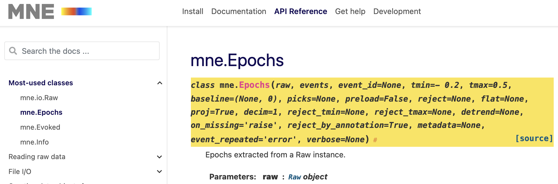
Overview: Epoching continuous data
epochs = mne.Epochs(raw, events, event_id=event_dict, tmin=-0.2, tmax=0.5,
                    reject=reject_criteria, preload=True)
Not setting metadata319 matching events foundSetting baseline interval to [-0.19979521315838786, 0.0] secApplying baseline correction (mode: mean)Created an SSP operator (subspace dimension = 4)4 projection items activatedLoading data for 319 events and 106 original time points ... Rejecting epoch based on EEG : ['EEG 001', 'EEG 002', 'EEG 003', 'EEG 007'] Rejecting epoch based on EOG : ['EOG 061'] Rejecting epoch based on MAG : ['MEG 1711'] Rejecting epoch based on EOG : ['EOG 061'] Rejecting epoch based on EOG : ['EOG 061'] Rejecting epoch based on MAG : ['MEG 1711'] Rejecting epoch based on EEG : ['EEG 008'] Rejecting epoch based on EOG : ['EOG 061'] Rejecting epoch based on EOG : ['EOG 061'] Rejecting epoch based on EOG : ['EOG 061']10 bad epochs dropped
Overview: Epoching continuous data
conds_we_care_about = [
  'auditory/left',
  'auditory/right',
  'visual/left',
  'visual/right']

# this operates in-place
epochs.equalize_event_counts(conds_we_care_about)

aud_epochs = epochs['auditory']
vis_epochs = epochs['visual']

del raw, epochs  # free up memory
Dropped 7 epochs: 121, 195, 258, 271, 273, 274, 275- Finer points for selection of conditions:
- Selecting part of a slashed event_id allows additional flexibility
- Forward-slash operator enables parts of event_id to act independently
- Assigning first part alone (aud or vis) combines both left and right
- Term order doesn’t matter (e.g., for left or right)

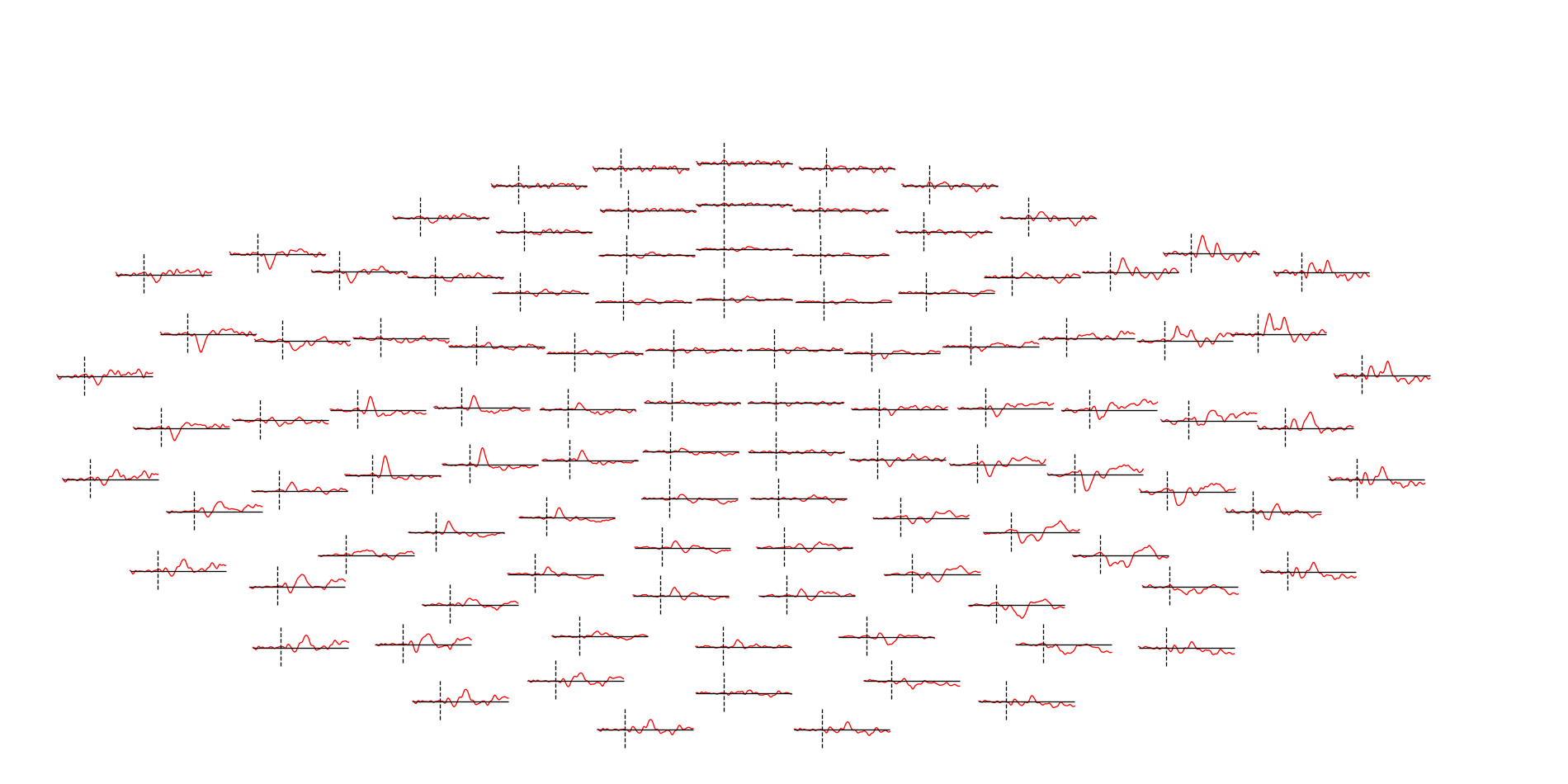
Overview: Epochs Plot-types
- MNE: pick and select
- Pick channels and data types
- Slice and select epochs
- Copy and Crop time epoch segments
Note
It’s important to select the specific data that you want to plot. MNE often will ‘try’ to plot all the data that you throw at it.
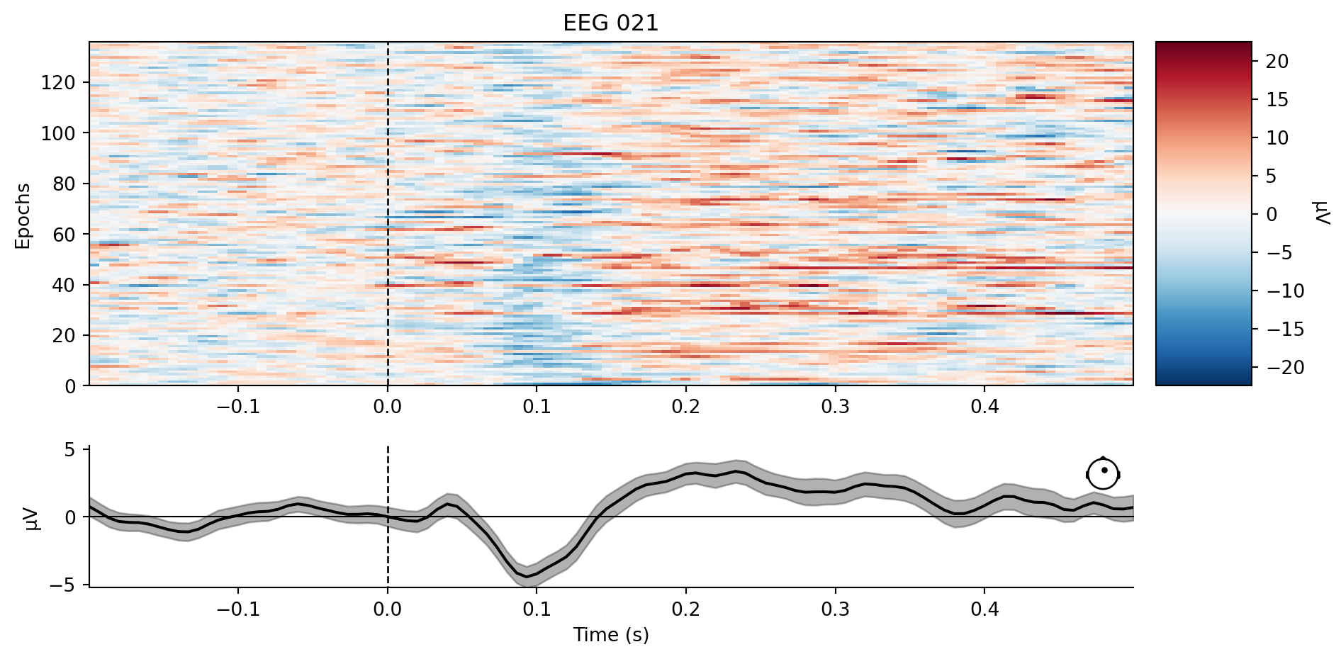
Overview: Time-frequency analysis
Removing projector <Projection | PCA-v1, active : True, n_channels : 102>Removing projector <Projection | PCA-v2, active : True, n_channels : 102>Removing projector <Projection | PCA-v3, active : True, n_channels : 102>Removing projector <Projection | PCA-v1, active : True, n_channels : 102>Removing projector <Projection | PCA-v2, active : True, n_channels : 102>Removing projector <Projection | PCA-v3, active : True, n_channels : 102>No baseline correction applied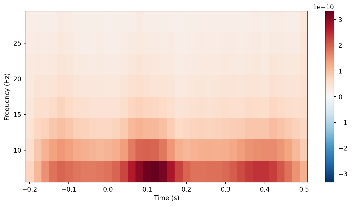
[<Figure size 960x480 with 2 Axes>]Overview: Estimating evoked responses
<Evoked | '0.50 × auditory/left + 0.50 × auditory/right' (average, N=136), -0.1998 – 0.49949 sec, baseline -0.199795 – 0 sec, 366 ch, ~3.6 MB>
Overview: Estimating evoked responses
mne.viz.plot_compare_evokeds(dict(auditory=aud_evoked, visual=vis_evoked),
                             legend='upper left', show_sensors='upper right')
Multiple channel types selected, returning one figure per type.combining channels using "gfp"combining channels using "gfp"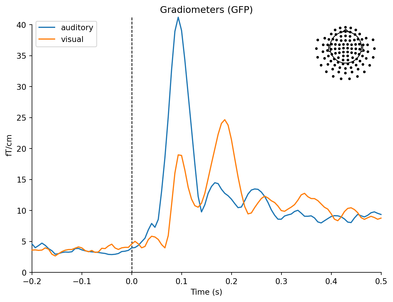
combining channels using "gfp"combining channels using "gfp"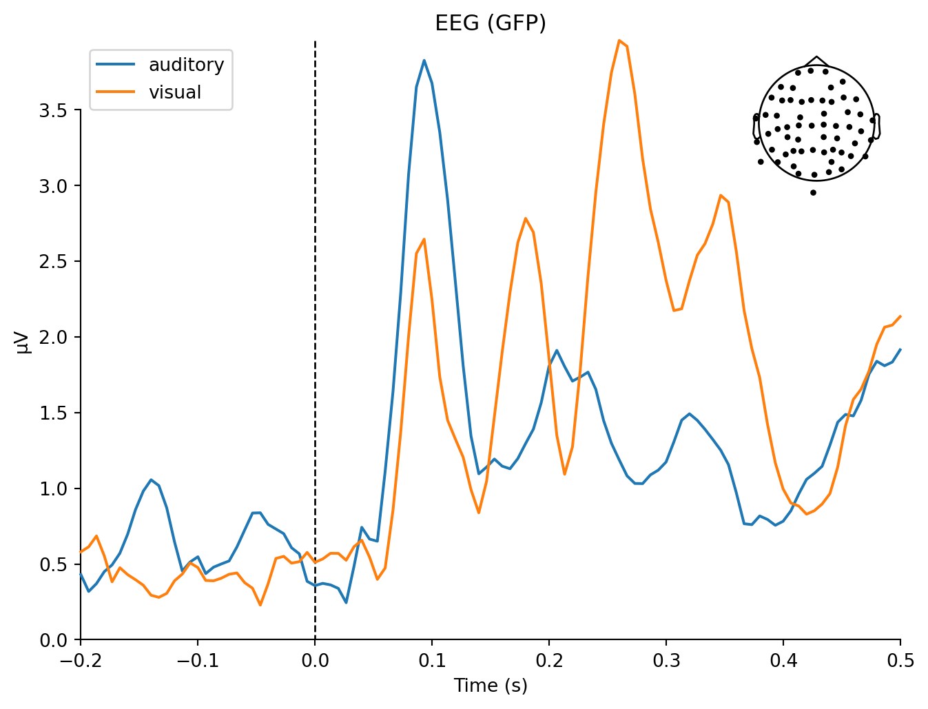
combining channels using "gfp"combining channels using "gfp"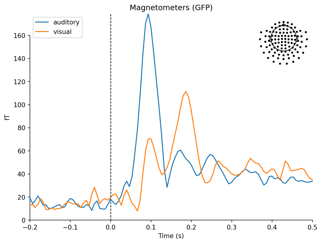
[<Figure size 768x576 with 2 Axes>,
 <Figure size 768x576 with 2 Axes>,
 <Figure size 768x576 with 2 Axes>]
Overview: Estimating evoked responses
Projections have already been applied. Setting proj attribute to True.Removing projector <Projection | PCA-v1, active : True, n_channels : 102>Removing projector <Projection | PCA-v2, active : True, n_channels : 102>Removing projector <Projection | PCA-v3, active : True, n_channels : 102>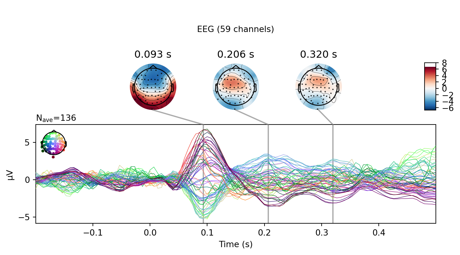

Overview: Estimating evoked responses

Python Tip
Lists are created by list() or by ‘[]’ literals.
Overview: Estimating evoked responses
<Evoked | '(0.50 × auditory/left + 0.50 × auditory/right) - (0.50 × visual/left + 0.50 × visual/right)' (average, N=68.0), -0.1998 – 0.49949 sec, baseline -0.199795 – 0 sec, 366 ch, ~3.6 MB>
Overview: Estimating evoked responses
Removing projector <Projection | Average EEG reference, active : True, n_channels : 60>